Schelling’s Model of Housing Segregation¶

Due: Friday, October 19th at 4pm

The goal of this assignment is to give you practice using nested loops, lists of lists, and functions.

You may work alone or in a pair on this assignment. The algorithms you need to implement for this assignment are more challenging than the first assignment. We recommend starting early.

Introduction¶

The New York Times has an interesting tool for viewing the distribution of racial and ethnic groups in cities and states around the country. If you look at the map for the Greater Chicago area, you will see that many areas are heavily segregated, but that some, such as the suburb of Glendale Heights, are not. The forces that led to this arrangement of people are complex and it is unlikely that any simple model can truly answer the questions of how segregation arises and why it persists. Keeping that in mind, one can still ask simple questions that may shed some light on the situation. In his 1978 book Micromotive and Macrobehavior, Thomas Schelling considered the following question: is it possible that a group of individuals would prefer to live in integrated neighborhoods and yet, as the result of their collective choices end up in segregated neighborhoods?

Schelling examined this question using a very simple model: A city has two kinds of people, Cubs fans and White Sox fans, for example, and each person in the city requires a certain number of their neighbors to be like them to feel comfortable in their location. Schelling used this model to study the patterns that emerge if, over time, people who are unsatisfied with their initial locations or become unsatisfied over time relocate to new locations that satisfy their criteria. What happens depends on the ratio of the two populations and on the satisfaction criteria used by the individuals, but segregation is a frequent outcome.

Schelling’s model of housing discrimination has led to myriad follow-up work examining different facets of the model’s outcomes in different circumstances, as well as applying the model to longitudinal datasets of urban environments. Data about Chicago features in a number of these analyses.

Our Model¶

Your task in this assignment will be to implement a variant of Schelling’s model. Before you can do so, we need to specify the details of the model. In particular, we need to specify the:

shape and composition of a city,
boundaries of a home’s neighborhood,
color of homeowners and criteria for similarity,
definition for satisfaction,
rule for relocating homeowners,
composition of a step in the simulation, and
stopping conditions for the simulation.

Cities: A city is represented as an $N \times N$ grid (where the value of $N$ can be different for each city). Each grid location (or cell) represents a home, which can be either open (that is, unoccupied) or occupied by a homeowner. As discussed below, each homeowner is indicated by one of two colors. You may assume that a city has at least one open location.

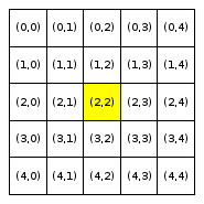
Neighborhood: The neighborhood of a home will be defined by a parameter R (this radius value will be an input to the model, so the value of R may vary from one simulation to another). The R-neighborhood of the home at Location $(i,j)$ contains all Locations $(k,l)$ such that:

$0 \le k \lt N$ and $i-R \le k \le i+R$
$0 \le l \lt N$ and $j-R \le l \le j+R$

Note that the Location $(i,j)$ itself is considered part of its own neighborhood. Thus, every homeowner will have at least one neighbor (themselves).

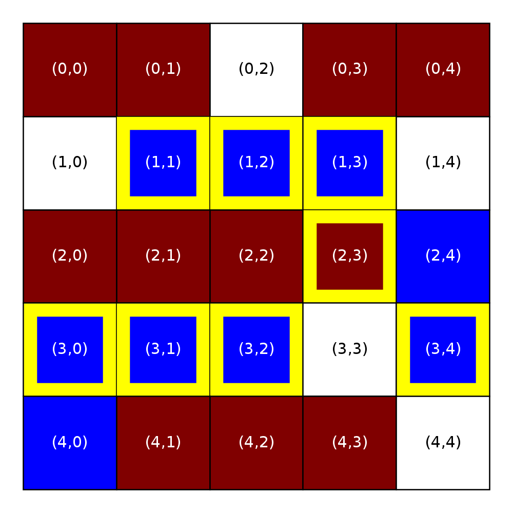
We will refer to a neighborhood with parameter R=x as an “R-x neighborhood”. The following figure shows the neighborhoods around Locations (2,2) and (3,0) for different values of R. Cells colored yellow are included in the specified neighborhood.

Neighborhood around (2,2)		Neighborhood around (3,0)
R = 0	R = 1	R = 1	R = 2

Notice that Location (3,0), which is closer to the boundaries of the city, has fewer neighboring homes for the same value of R than Location (2,2), which is the middle of the city. We use the term boundary neighborhood to refer to a neighborhood that is near the boundary of the city and thus does not have a full set of neighbors.

Color of homeowner and definition of similarity: We define two groups of homeowners: maroon homeowners and blue homeowners. Homeowners of a particular group prefer to live in a neighborhood where at least some given fraction of their neighbors are from the same group as them. That is, maroon homeowners prefer that at least some minimum fraction of their neighbors are also maroon, while blue homeowners prefer that at least some minimum fraction of their neighbors are also blue. In Schelling’s original model, all homeowners had identical preferences to other homeowners. However, more recent work by two groups of researchers – Xie and Zhou and Hatna and Benenson – has explored heterogeneity in preferences among homeowners of a given group. In this assignment, we will consider a model that partially accounts for heterogeneity.

Throughout the assignment, maroon homeowners will be indicated with an M while blue homeowners will be indicated with a B.

Satisfaction: For each homeowner, we are going to compute a similarity score to determine whether they are satisfied. We define the similarity score to be S/H where S is the number of homes in the neighborhood with occupants of the same color as the homeowner and H is the number of occupied homes in the neighborhood.

Since a homeowner is included in their own neighborhood, S will always be at least one and H will be at least one. A homeowner is satisfied with their location if their similarity score is greater than or equal to a specified threshold. In our partially heterogeneous model, the satisfaction thresholds for maroon homeowners and blue homeowners will sometimes be different. We term the satisfaction threshold for maroon homeowners the M threshold and the satisfaction threshold for blue homeowners the B threshold.

The figure below illustrates this concept using a city with R-1 neighborhoods. It shows homeowners and their similarity scores. White cells depict unoccupied homes/locations. Cells that are maroon (dark red) contain maroon homeowners. Cells that are blue contain blue homeowners. Each grid cell contains its location (in parentheses) and, for occupied homes, the homeowner’s R-1 similarity score (in square brackets). We rounded the similarity scores in the figure to three digits merely for clarity. Do not round them in your computation.

Similarity scores
R=1

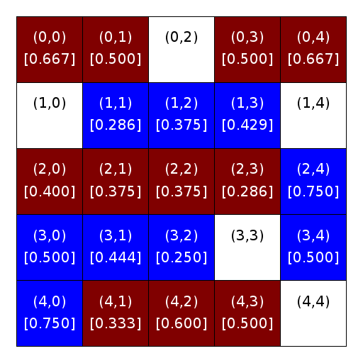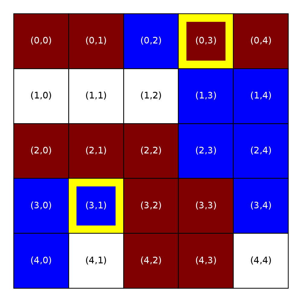
We will first set both satisfaction thresholds – the M threshold and the B threshold – at 0.33. We will then determine which homeowners are satisfied, and which are not. Throughout this assignment, we indicate unsatisfied homeowners with a yellow border.

Satisfaction
R=1
M Threshold = B Threshold = 0.33

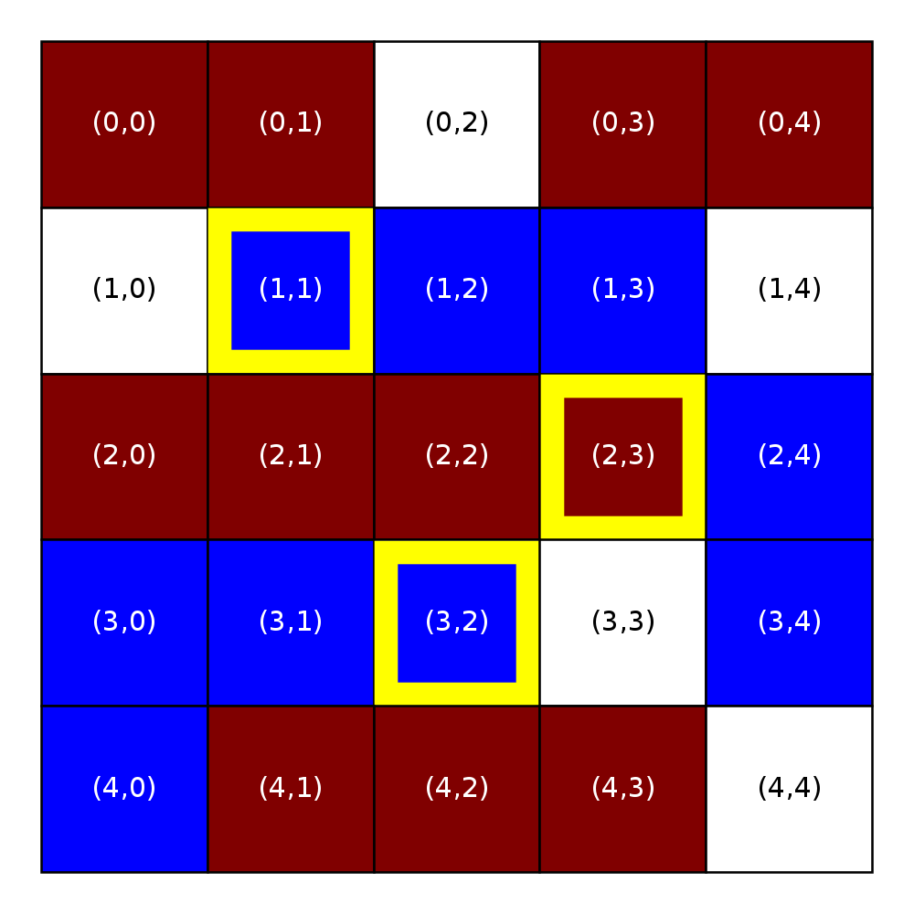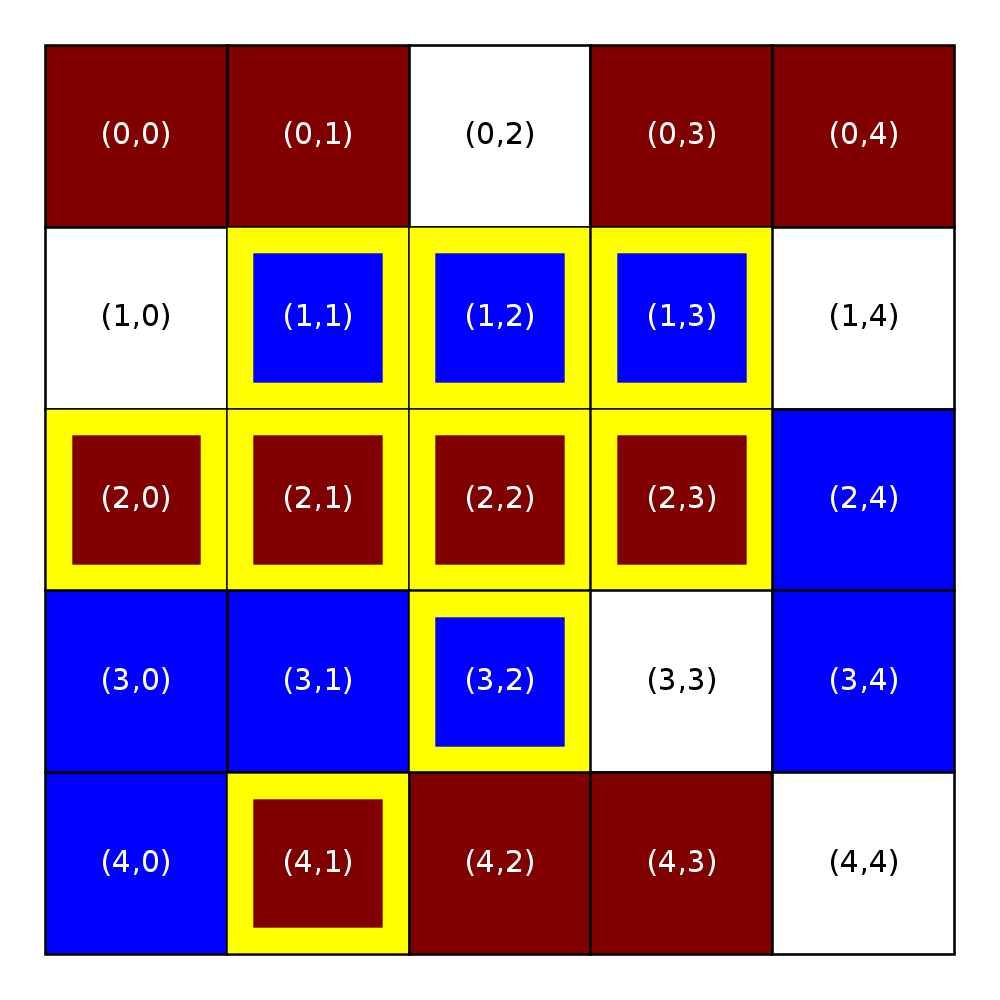
The next two figures will illustrate the impact of the threshold on satisfaction. The figure on the left was computed using an M threshold and a B threshold both set at 0.33. The figure on the right, however was computed using both thresholds set at 0.60. As in the figures above, white locations are unoccupied.

M threshold = 0.33	M threshold = 0.60
B threshold = 0.33	B threshold = 0.60
R=1	R=1

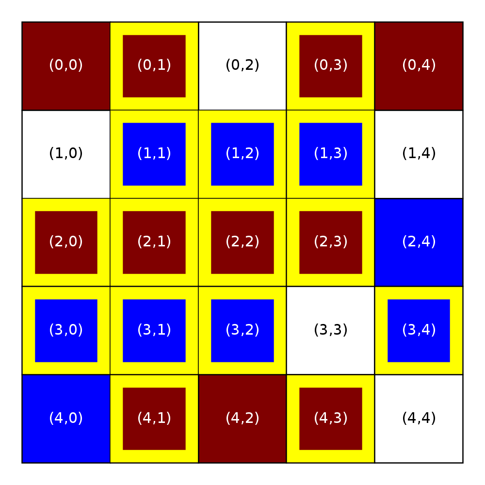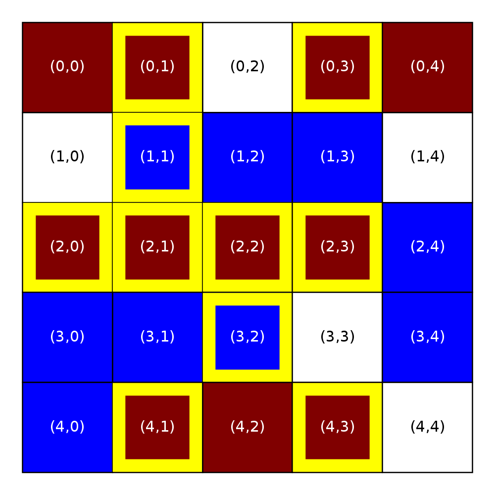
Next, we will further illustrate the impact of the threshold on satisfaction through two examples in which the M and B thresholds are different.

M threshold = 0.33	M threshold = 0.60
B threshold = 0.60	B threshold = 0.33
R=1	R=1

Relocation rule: Homeowners always want to live in a satisfactory location. If possible, an unsatisfied homeowner should be relocated to an open location that would meet the satisfaction criteria. To determine whether a prospective new location would be acceptable, temporarily swap the homeowner to that prospective new location, calculating whether the homeowner would be satisfied in that new location.

Complicating matters, our homeowners are picky: they want to move to satisfactory locations, but would prefer to stay close to their old neighborhood. Therefore, they will move to the satisfactory home that is closest to their old home. Calculate the distance between ($r_{1}$, $c_{1}$) and ($r_{2}$, $c_{2}$) using the standard Euclidean distance:

\[Distance = \sqrt{(r_{2} - r_{1})^{2} + (c_{2} - c_{1})^{2}}\]

For example, the distance between (2,2) and (4,2) on the grid is $2$. The distance between (2,2) and (3,3) is $\sqrt{2}$. Hint: while Python does have a square root function in the math module (which you have not learned about yet), you can also calculate square roots using only operators you already know, such as raising a value to the 0.5 power. Note that if a homeowner’s current home is already satisfactory, then that is where they wish to live because the home is satisfactory and the distance from their previous home is 0. That is, a homeowner will not move from a home that is already satisfactory.

However, sometimes homeowners will have multiple homes to choose from at the same (closest) distance. In these cases, homeowners prefer to move into more vibrant neighborhoods with more neighbors. That is, as a tiebreaker between satisfactory homes that are equally close, the homeowner will prefer the home that has more direct neighbors. We define direct neighbors as the number of occupied homes that would be in the new location’s R-1 neighborhood if the homeowner were to move there. Following the earlier definition of neighborhoods, there will always be at least one direct neighbor (the homeowner themselves). For homes near the boundary of the city, you may assume that there are no direct neighbors outside the boundary of the city. Finally, as a second tiebreaker, because homeowners assume that a home that has been vacant for a while might suffer from issues, the homeowner will prefer homes that have been unoccupied for the shortest amount of time.

To state these preferences more precisely: given multiple (unoccupied) homes that meet the satisfaction threshold, an unsatisfied homeowner will choose the closest home (the home with the minimum distance from the homeowner’s current location). In the case of ties, the first tiebreaker will be to select the home with the most direct neighbors from among those that are equally close. If there is still a tie, the homeowner will choose the home that has been on the market shortest from among those remaining. For the sake of computational efficiency, compute the values needed for these tiebreakers only when necessary. If none of the available homes are satisfactory, however, then the homeowner will not relocate.

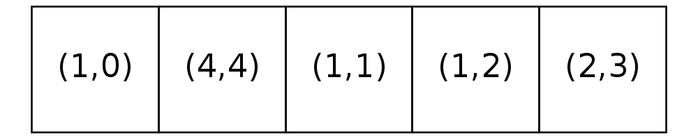
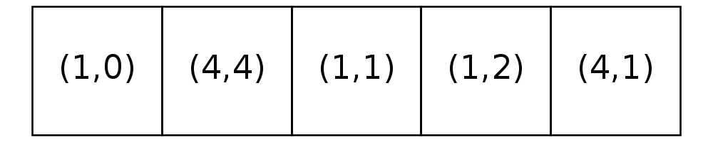
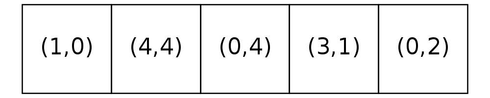
We will model the homes that are currently available with a list of their locations. Once a homeowner chooses a home, the location of their new home should be removed from the list and the location of their previous home should be added to the end of the list of available homes. That is, we will be keeping this list of homes in order from oldest listing to newest listing.

Note that you should determine the best location for a homeowner using a single pass through the list of open locations. As you move through the list, we suggest that you keep track of the move that is the “best so far” among those you have seen at that point iterating through the list.

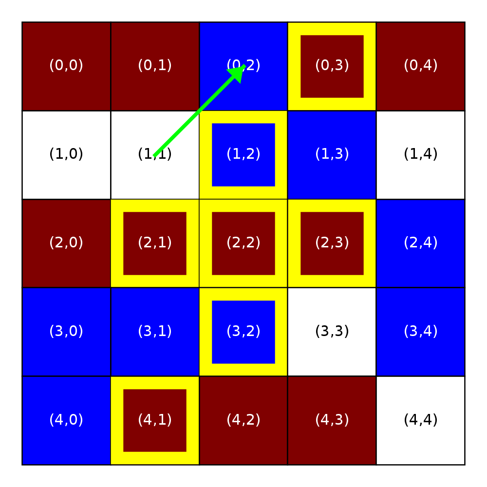
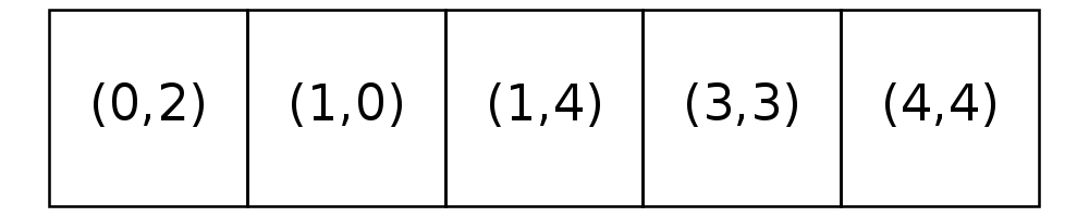
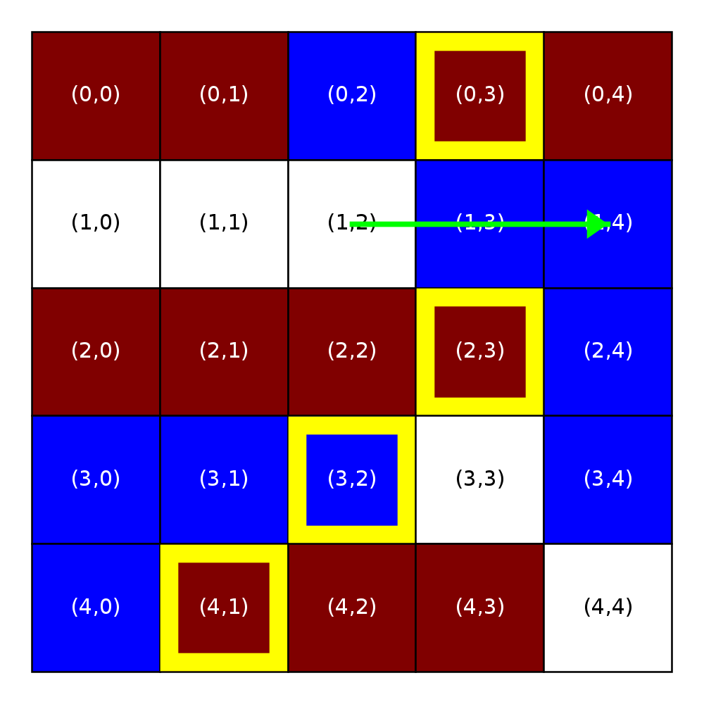
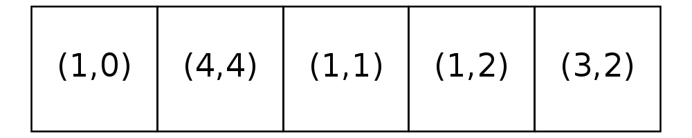
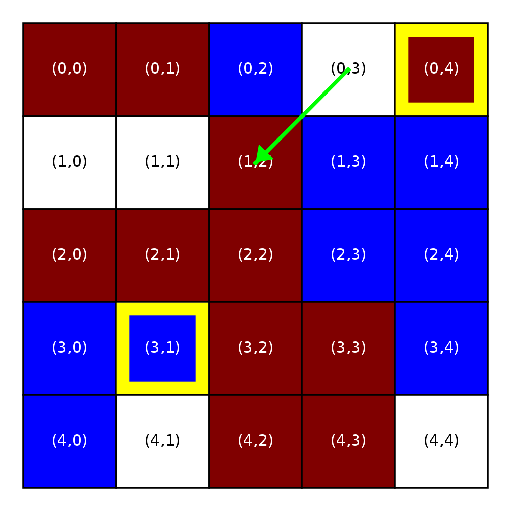
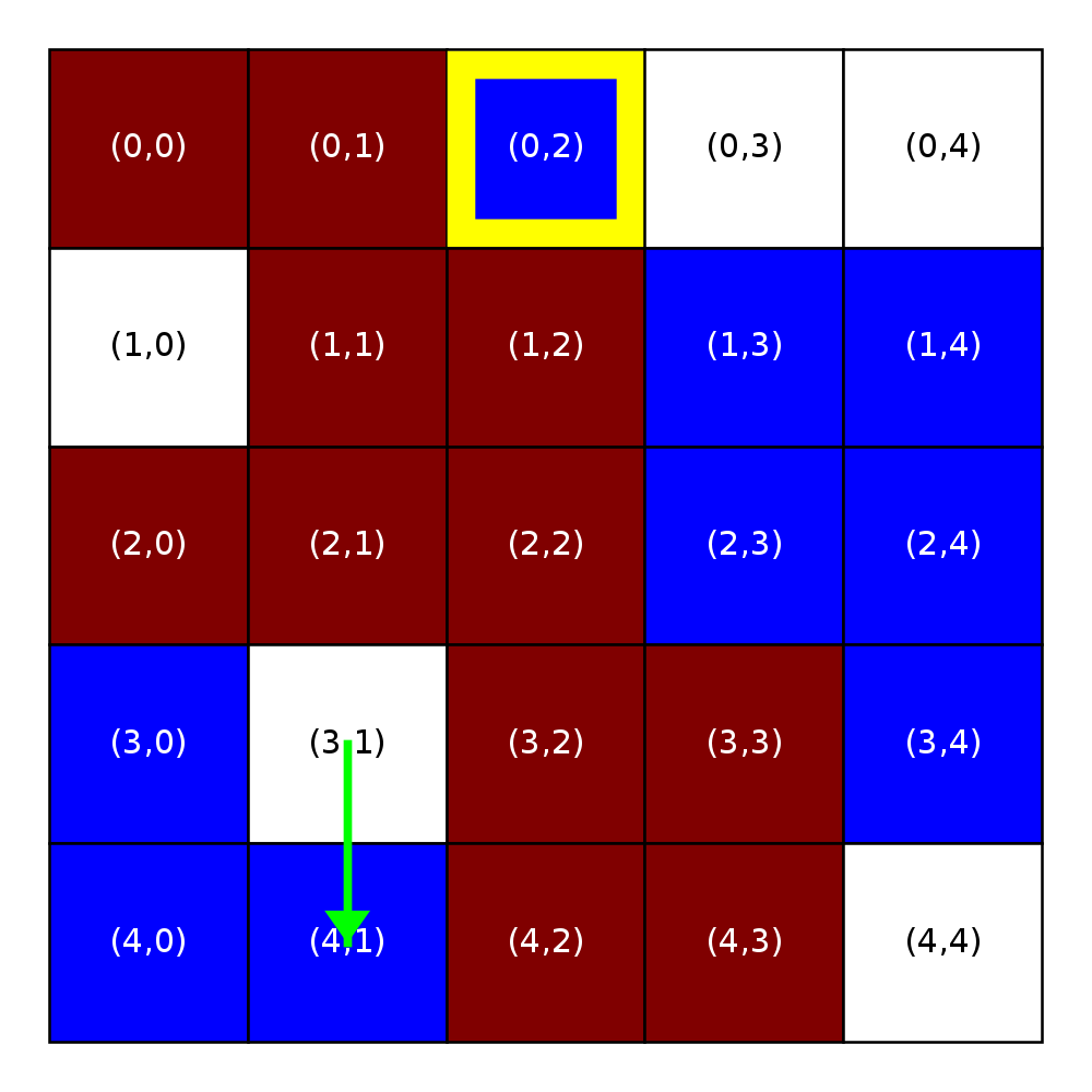
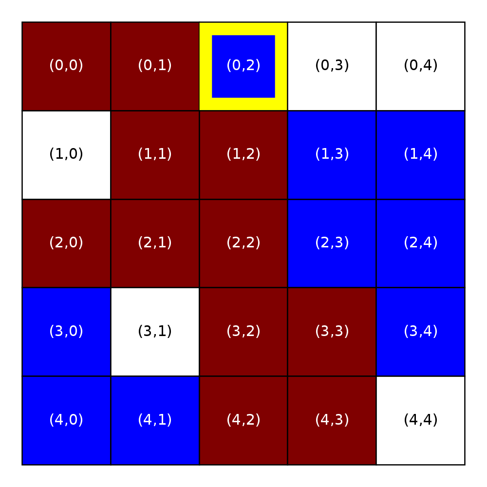
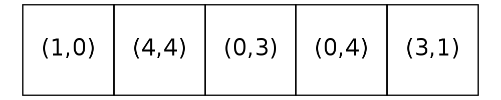
Here is an example relocation of the unsatisfied homeowner at Location (1,1) to Location (0,2). On the left, we show a city with R-1 neighborhoods in which both the M threshold and B threshold are 0.44. Below the grid, we also include a depiction of the locations that are open in the neighborhood.

Before relocation	After relocation

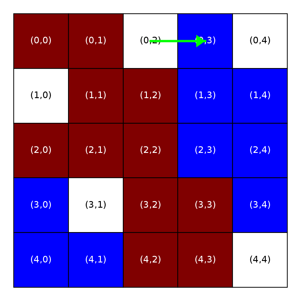
The blue homeowner in Location (1,1) is unsatisfied with their location. They consider all five open locations and find the following:

Location	Similarity Score (rounded to 3 decimal places)	Satisfactory	Distance (rounded to 3 decimal places)	# R-1 neighbors
Location (0,2)	0.6	Yes	1.414	5
Location (1,0)	0.2	No	1.0	5
Location (1,4)	0.5	Yes	3.0	6
Location (3,3)	0.5	Yes	2.828	8
Location (4,4)	0.667	Yes	4.243	3

Four of the locations – (0,2); (1,4); (3,3); (4,4) – have acceptable similarity scores. Therefore, the homeowner chooses among these four locations by choosing the one that is closest, which is (0,2) in this case. Had more than one of these locations been equally close, the homeowner would have preferred the location in the more vibrant neighborhood. Had there again been a tie, the homeowner would have moved to the location that had been on the market the shortest.

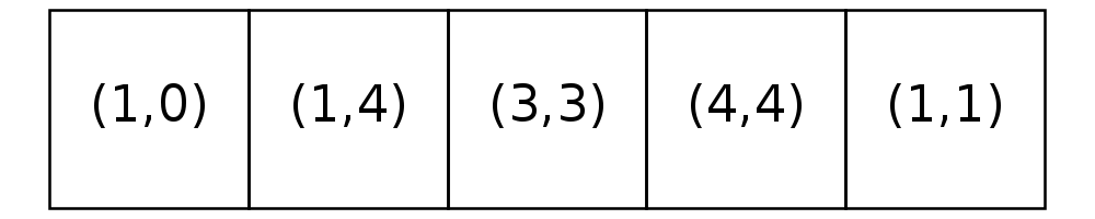
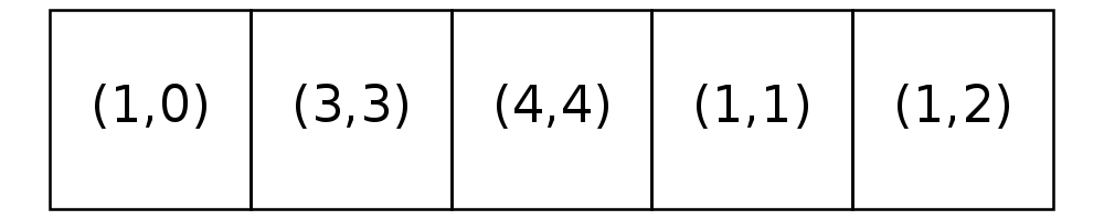
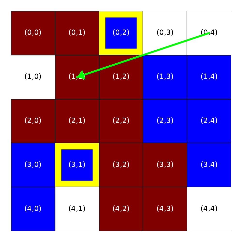
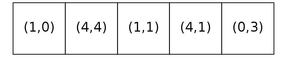
The frame on the right shows the state of the neighborhood after this homeowner has been relocated. Notice that location (0,2) has been removed from the list of open locations and location (1,1) has been added to the end of the list. Also, notice that the satisfaction states of the homeowners at locations (0,3) and (1,3) have changed. Can you figure out why?

Simulation Step: During a step in the simulation, your implementation should make a full pass over the city in row-major order. That is, you will use a doubly-nested loop in which the index variable in the outer loop starts at zero and is used to indicate the current row, and the index variable in the inner loop starts at zero and is used to indicate the current column.

As your implementation visits each home, you will check to see if the home is occupied and, if so, whether the homeowner is satisfied with their location at the time of the visit. If they are satisfied, then you will move on to the next home in the traversal. If not, you should attempt to relocate them to a more satisfactory location using the relocation rules described above.

To recap: a visit to a particular home will trigger a relocation in a given step if, at the time of the visit:

the home is occupied;
the homeowner is unsatisfied with their location; and
there is an open location that meets the satisfaction criteria.

Stopping conditions: Your simulation should stop when:

it has executed a specified maximum number of steps or
no relocations occur in a step.

Sample simulation: Step 1

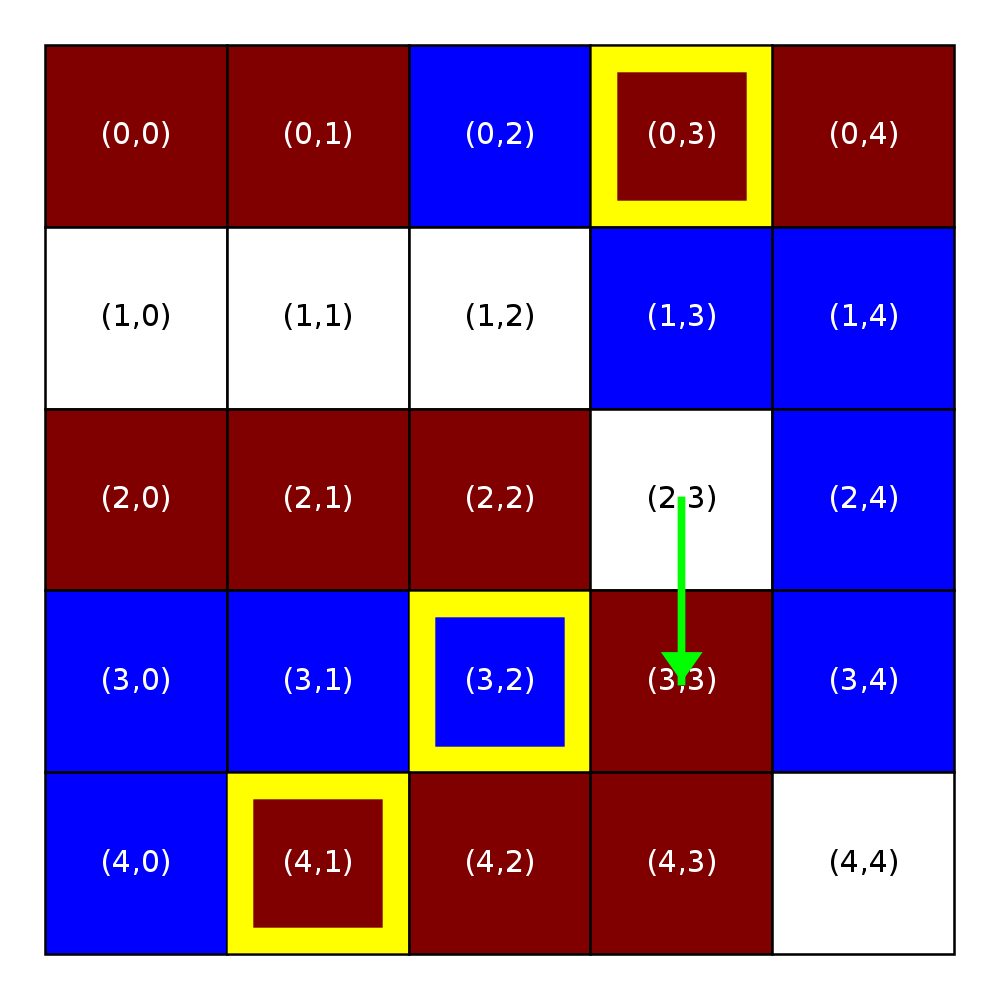
Continuing the example above, we will simulate a city with R-1 neighborhoods and both thresholds (M threshold and B threshold) set at 0.44. In the figure below, the first frame represents the initial state of a city. The next five frames illustrate the relocations that occur in the first step of the simulation.

Step 1
Initial state	After 1st relocation	After 2nd relocation


After 3rd relocation	After 4th relocation	After 5th relocation

At the start of step 1, all of the homeowners in row 0 (that is, in Locations (0,0), (0,1), (0,3), and (0,4)) are satisfied. The homeowner in location (1,1) is the first unsatisfied homeowner encountered during our traversal of the city. As discussed above in the relocation example, the homeowner will move to location (0,2).

Relocating the blue homeowner at location (1,1) causes the maroon homeowner at location (0,3) to become unsatisfied. However, because we have already passed this location in our row-major traversal during the current step, we will not consider moving the homeowner at location (0,3) until the next step.

The next homeowner in our row-major traversal is at location (1,2). That homeowner is an unsatisfied blue homeowner. The closest satisfactory location is (1,4), so they move there.

The next homeowner is then the homeowner at location (1,3). While, earlier in this step, this blue homeowner had been unsatisfied, the first relocation conveniently caused them to become satisfied. Because we consider moving only those homeowners who are unsatisfied at the time they are visited in a step, we can move on to the next homeowner.

We next visit the homeowner in (1,4), whom we moved just a moment ago. They are now satisfied, so we move on. The next unsatisfied homeowner in our row-major traversal is then the maroon homeowner in (2,3). In this case, all five open locations are satisfactory, so the homeowner at location (2,3) moves to location (3,3) because it is closest.

The traversal continues through the rest of the locations in the grid, making a total of 5 relocations in this step. As of the initial state of this step, 9 homeowners were unsatisfied. At the end of this step, only 2 homeowners remain unsatisfied.

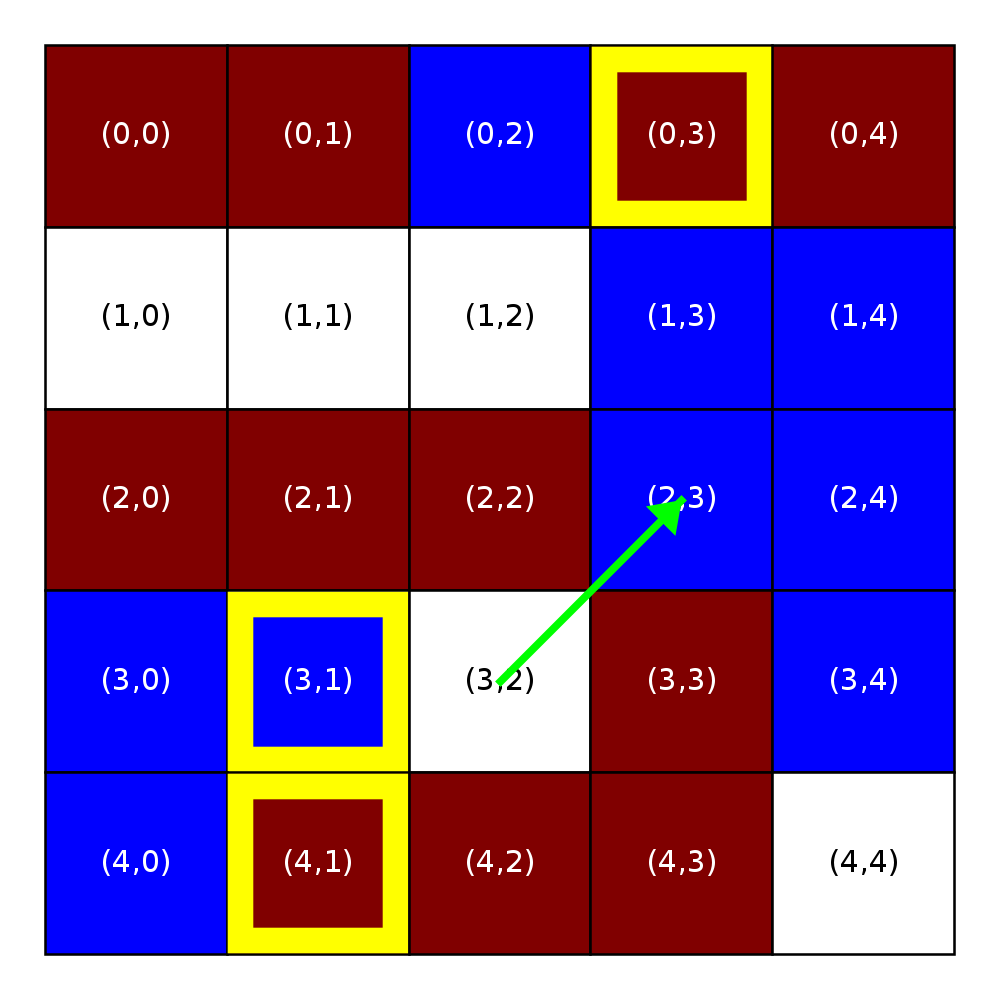
Sample simulation: Step 2

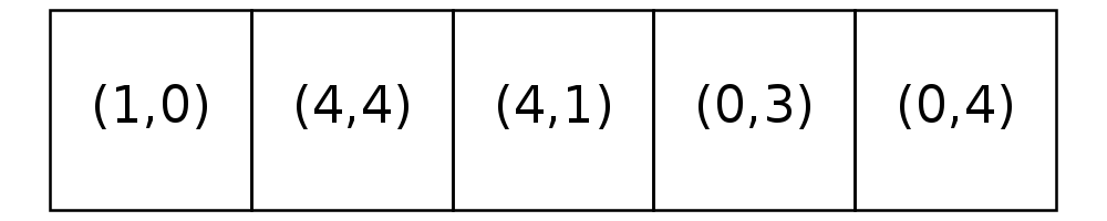
The first frame in the figure below represents the state of a city at the start of the second step. Notice that both the state of the grid and the open locations list are the same as they were at the end of the first step.

Step 2
Initial state	After 1st relocation	After 2nd relocation	After 3rd relocation

In Step 2 of the simulation, three relocations are made, as shown above. At the end of this step, however, the homeowner at location (0,2) has become unsatisfied as a result of the second relocation. As a result, a third step in the simulation is necessary (as long as the maximum number of steps has not yet been reached).

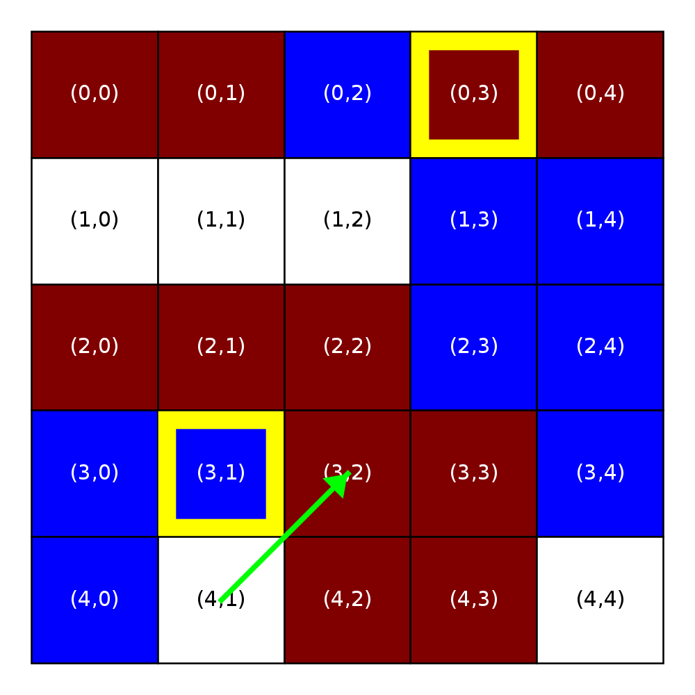
Sample simulation: Step 3

Step 3
Initial state	After 1st relocation	Final state

In Step 3, one relocation occurs. After this relocation, all homeowners are satisfied. As a result, no further relocations occur in this step.

Sample simulation: Step 4

Recall that there are two possible stopping conditions: one based on a specified maximum number of steps, and the other based on a step occurring without any relocations. As long as the specified number of steps has not been reached, Step 4 in this simulation will occur without any relocations, which would trigger the latter stopping condition and end the simulation.

Data representation¶

Your implementation will need a representation for the current state of a homeowner, a representation for the city (aka the grid), and a representation for the locations that are currently open (unoccupied).

Representing Homeowners/Homes: Homeowners will be represented by the strings “M” (maroon) and “B” (blue), and open homes are represented by “O” (the letter).

Representing cities: We will represent a city using a list of lists with strings as elements. You can assume that these strings will always be one of “M”, “B”, or “O”. Traversals of the city should always be done in row-major order.

The directory pa2/tests contains text representations of some sample city grids, including all of the grids shown above (see tests/a18-sample-writeup.txt). See the file tests/README.txt for descriptions of the grid file format and the grid files included in the tests sub-directory.

The file utility.py contains some functions that you might find useful when testing your code:

read_grid: takes the name of a grid file as a string and returns a grid. Here is a sample use that assumes utility has been imported:
```
utility.read_grid("tests/a18-sample-writeup.txt")
```
is_grid(grid): does grid have the right type and shape to be a city grid?
print_grid(grid): takes a grid and prints it to stdout.
find_mismatch(grid0, grid1): takes two grids and returns the first location at which they differ. This function returns None if the grids are the same.

You will be doing all of your development in the file schelling.py.

Representing Locations: We will use pairs (tuples) of integers to represent locations.

Tracking open locations We will use a list of pairs (locations) to track open locations. The initial list of open homes will be passed as a parameter to your simulation. All subsequent changes to the list will occur as the result of a relocation.

When looking for a new location for a homeowner, your implementation will walk through the list of open locations and consider them as possible new homes for the homeowner. If this process evaluating new homes for a homeowner determines that they should move to a new location, you should remove this location from the list (using del or remove) and append their old location to the end of the list (using append).

Note that when you consider a possible new home for a homeowner, you should not make a copy of the full grid because it would be computationally inefficient (involve extra computation) to do so. Instead, temporarily swap the homeowner into the proposed new home and set their current home to open, perform the necessary calculations, and then return the homeowner and to their initial location.

We encourage you to look carefully at the open locations list in the sample simulation above. In particular, notice that we do not recompute the list of open locations between steps.

Code structure¶

Your task is to implement in the file schelling.py a function:

def do_simulation(grid, R, M_threshold, B_threshold, max_steps, opens)

that executes simulation steps on the specified grid until one of the stopping conditions is met. This function must return the number of relocations done during the simulation. Your function can and should modify the grid argument. At the end of the simulation, the grid should reflect the relocations that took place during the simulation.

However, you should think carefully about how to split your tasks into multiple functions. That is, you will write a series of auxiliary functions (with appropriate function headers) that each implements a given subtask. When designing your function decomposition, keep in mind that you need to do the following subtasks:

determine whether a homeowner in a given location is satisfied; (We have already included a function header for the function is_satisfied for this purpose, though you will need to complete the function.)
calculate the distance between two locations;
calculate the number of R-1 direct neighbors;
swap the values at two locations;
evaluate open locations as potential new homes for a homeowner;
simulate one step of the simulation;
run steps until one of the stopping conditions is met.

Do not combine the last three tasks into one mega-task, because the resulting code would be hard to read and debug. You will lose significant style points if you have a mega-task.

Testing¶

We strongly encourage you to test your functions as you write them! The surest way to guarantee that you will need to spend hours debugging is to write all your code and only then start testing.

We have provided some test code for you, but you will also need to design some tests of your own.

Testing by hand

Recall that you can set-up ipython3 to reload code automatically when it is modified by running the following commands after you fire up ipython3:

%load_ext autoreload
%autoreload 2

and then loading the code for the first time:

import schelling, utility

Do NOT add the .py extension when you import schelling and utility.

Once you have done these tasks, you can test your code by hand: simply read a grid from a file and then call the function with the appropriate arguments.

For example, if you wanted do a few quick tests of your function to determine whether a homeowner in a given location is satisfied (your is_satisfied function), you could do something like the following:

grid = utility.read_grid("tests/a18-sample-writeup.txt")
schelling.is_satisfied(grid, 0, (0, 0), 0.3, 0.7)   # expected result: True
schelling.is_satisfied(grid, 2, (0, 0), 0.8, 0.9)   # expected result: False

The function is_satisfied does not modify the grid and so, it is not necessary to reload the grid between tests. On the other hand, the grid does need to be reloaded when testing do_simulation:

grid = utility.read_grid("tests/a18-sample-writeup.txt")
opens = utility.find_opens(grid)
schelling.do_simulation(grid, 1, 0.44, 0.44, 1, opens)  # do one step

grid = utility.read_grid("tests/a18-sample-writeup.txt")
opens = utility.find_opens(grid)
schelling.do_simulation(grid, 1, 0.44, 0.44, 4, opens)  # do all four steps.

Testing satisfaction function

To encourage you to separate out the task of determining whether a homeowner is satisfied, we have provided test code for such a function. Our code assumes that you have written a function with the header:

def is_satisfied(grid, R, location, M_threshold, B_threshold):

that computes whether the homeowner is satisfied at the specified location for neighborhood defined by R and the M_threshold and B_threshold provided.

For each test case, our test code reads the input grid from a file, calls your is_satisfied function with the grid and the other parameters specified for the test case, and checks the actual result against the expected result. Here is a description of the tests:

Tests for `is_satisfied`¶
Test number	Grid filename	R	Location	M threshold	B threshold	Expected result	Similarity score	Purpose
0	tests/a18-sample-grid.txt	0	(0, 4)	0.8	0.9	True	1.000000	Check boundary neighborhood: top right corner.
1	tests/a18-sample-grid.txt	1	(0, 4)	0.7	0.8	False	0.666667	Check boundary neighborhood: top right corner.
2	tests/a18-sample-grid.txt	2	(0, 4)	0.5	0.55	True	0.666667	Check boundary neighborhood: top right corner.
3	tests/a18-sample-grid.txt	0	(4, 0)	0.9	0.95	True	1.000000	Check boundary neighborhood: lower left corner.
4	tests/a18-sample-grid.txt	1	(4, 0)	0.8	0.85	True	1.000000	Check boundary neighborhood: lower left corner.
5	tests/a18-sample-grid.txt	2	(4, 0)	0.4	0.5	True	0.833333	Check boundary neighborhood: lower left corner and difference between M and B thresholds.
6	tests/a18-sample-grid.txt	0	(1, 1)	0.3	0.7	True	1.000000	Check interior R-0 neighborhood.
7	tests/a18-sample-grid.txt	1	(1, 1)	0.2	0.25	True	0.666667	Check neighborhood that is complete when R is 1.
8	tests/a18-sample-grid.txt	2	(1, 1)	0.9	0.9	False	0.727273	Check neighborhood that is not complete when R is 2 and difference between M and B thresholds.
9	tests/a18-sample-grid.txt	2	(2, 3)	0.5	0.6	True	0.666667	Check neighborhood that corresponds to the whole city.
10	tests/grid-no-neighbors.txt	1	(2, 2)	0.2	0.7	True	1.000000	Check interior neighborhood with location that has no other neighbors.
11	tests/grid-no-neighbors.txt	1	(4, 4)	0.5	0.7	True	1.000000	Check boundary neighborhood (lower right corner) with location that has no other neighbors.
12	tests/grid-no-neighbors.txt	2	(4, 4)	0.3	0.4	False	0.250000	Check boundary neighborhood (lower right corner) with location that has a few neighbors.

Please keep in mind that even though there are many corner cases for this function, your code does not need to be complex! Our function, excluding the header comment, is roughly 15 lines of code.

As in PA #1, we will be using py.test to test your code. You can run our is_satisfied tests from a Linux terminal window with the command:

$ py.test -xv test_is_satisfied.py

(As in PA #1: we will use $ to signal the Linux command-line prompt.)

Recall that the -x flag indicates that pytest should stop when a test fails. The -v flag indicates that pytest should run in verbose mode. And the -k flag allows you to reduce the set of tests that is run. For example, using -k test_0 will only run the first test.

Testing the full simulation

We have also provided test code for do_simulation. For each test case, our code reads in the input grid from a file, calls your do_simulation function, checks the actual state of the grid against the expected state of the grid, and checks the actual number of relocations returned by do_simulation against the expected number of relocations.

Here is a description of the tests:

Tests for `test_do_simulation`¶
Test number	Input grid filename	Expected grid filename	R	M Threshold	B Threshold	Maximum number of steps	Expected numer of relocations	Purpose
0	tests/a18-sample-grid.txt	tests/a18-sample-grid-1-33-33-0-final.txt	1	0.33	0.33	0	0	Check stopping condition #1
1	tests/a18-sample-grid.txt	tests/a18-sample-grid-1-33-33-3-final.txt	1	0.33	0.33	3	2	Check stopping condition #2
2	tests/a18-sample-grid.txt	tests/a18-sample-grid-1-60-40-1-final.txt	1	0.60	0.40	1	5	Check choosing among acceptable locations.
3	tests/a18-sample-grid.txt	tests/a18-sample-grid-1-60-40-2-final.txt	1	0.60	0.40	2	6	Check choosing among acceptable locations.
4	tests/grid-sea-of-red.txt	tests/grid-sea-of-red-1-40-70-1-final.txt	1	0.40	0.70	1	0	Check case where there are no suitable homes.
5	tests/a18-sample-grid.txt	tests/a18-sample-grid-1-75-25-1-final.txt	1	0.75	0.25	1	6	Check case where possible new location is in the homeowner’s current neighborhood.
6	tests/a18-sample-grid.txt	tests/a18-sample-grid-1-30-50-1-final.txt	1	0.30	0.50	1	5	Check that the different thresholds are recognized.
7	tests/a18-sample-grid.txt	tests/a18-sample-grid-1-50-30-1-final.txt	1	0.50	0.30	1	2	Check that the different thresholds are recognized.
8	tests/a18-sample-grid.txt	tests/a18-sample-grid-2-44-70-7-final.txt	2	0.44	0.7	7	0	Check sample grid with R of 2.
9	tests/grid-ties.txt	tests/grid-ties-2-33-70-2-final.txt	2	0.33	0.70	2	4	Check choosing among equidistant locations.
10	tests/grid-ten.txt	tests/grid-ten-2-40-65-2-final.txt	2	0.40	0.65	2	21	Check whether more recently vacant homes are preferred.
11	tests/grid-ten.txt	tests/grid-ten-2-32-62-4-final.txt	2	0.32	0.62	4	23	Check 4 steps of a medium-size grid.
12	tests/grid-ten.txt	tests/grid-ten-3-32-62-4-final.txt	3	0.32	0.62	4	1	Check a larger R.
13	tests/large-grid.txt	tests/large-grid-2-33-70-20-final.txt	2	0.33	0.70	20	188	Check a large grid.

You can run the following command from a Linux terminal window:

$ py.test -xv -k "not large" test_do_simulation.py

to run all the tests except the one that uses the large grid. We encourage you to run the large test only after you have successfully passed all the small tests! To do so, remove -k “not large” from the command above.

Running your program¶

The run function is the “main function” supplied in schelling.py that parses the command-line arguments, reads a grid from a file, calls your do_simulation function, and if the grid is small, it prints the resulting grid.

The command line arguments are: the name of the input grid file, a value for R, values for the two satisfaction thresholds, and a maximum number of steps. For example, running the following command from the Linux terminal window:

$ python3 schelling.py --grid_file=tests/a18-sample-writeup.txt --r=1 --m_threshold=0.44 --b_threshold=0.44 --max_steps=1

will do a simulation using the grid specified in the file tests/a18-sample-writeup.txt, with R=1, an M threshold of 0.44, a B threshold of 0.44, and a maximum number of steps of 1.

Grading¶

Programming assignments will be graded according to a general rubric. Specifically, we will assign points for completeness, correctness, design, and style. (For more details on the categories, see our PA Rubric page.)

The exact weights for each category will vary from one assignment to another. For this assignment, the weights will be:

Completeness: 50%
Correctness: 15%
Design: 20%
Style: 15%

The design score will be largely based on how you decompose the problem into multiple functions. You will receive a zero in this section if you implement your entire code inside the do_simulation function. Your must break up this problem into more manageable pieces, and write functions that address each of those sub-problems.

Because the tests only check the is_satisfied and do_simulation functions, the correctness score will be largely based on how you implement the other functions in your solution. For example, if you design a function that claims to produce a particular result, and that function happens to make the tests pass but could fail under other reasonable conditions, we would deduct points for this. For example, if you claim that a given function returns False if certain conditions are met, but you’re not checking all those conditions (or we can come up with a reasonable counter-example where the function returns a value other than the one specified in the function documentation), we would deduct points for this.

Finally, since you are writing your own functions, you must include header comments in all of your functions (and you must make sure they conform to the format specified in the style guide). A large portion of the Style section will be allocated to this.

Obtaining your test score¶

Like PA1, you can obtain your test score by running py.test followed by ../common/grader.py.

Continuous Integration¶

Continuous Integration (CI) is available for this assignment. For more details, please see our Continuous Integration page. We strongly encourage you to use CI in this and subsequent assignments.

Getting started/Submission¶

See these start-up and submission instructions if you intend to work alone.

See these start-up and submission instructions if you intend to work in a pair.

Acknowledgments: This assignment was inspired by a discussion of Schelling’s Model of Segregation in Housing in the book Networks, Crowds, and Markets by Easley and Kleinberg.