![[back]](http://cs-www.uchicago.edu/images/logos/UofCsealTiny.gif) Department of Computer Science
The University of Chicago
Department of Computer Science
The University of Chicago
Last modified: Fri Jan 22 11:25:27 CST 1999
It might be surprising to find that the chapter on ``Fundamentals of Computer Design'' has very little technical information about computer design, but a lot of information on cost, price, and performance measures. Perhaps the chapter title isn't perfect, but it is very sensible to start out with this sort of information. In some areas of engineering, economic forces and techniques are stable enough that one can study a problem in terms of the most effective way to meet some specified requirements. In the computer business, the techniques available to the designer, and the economic forces on her, change so rapidly that the rate of change becomes as important as the current state. Essentially every decision in the computing business has to be made based on some estimate of the changes that will occur before it takes effect.
Please read all of chapter 1 in the text, but you needn't focus equal attention everywhere. Skim through 1.1-1.3, and don't worry too much about the jargon. Notice that ``technology'' usually means electronics in this sort of text. Focus on the rates of change described for various parameters, such as 60%-80% increase per year in transistors on a chip.
Pay closer attention to 1.4, particularly the section on ``Cost of an Integrated Circuit.'' The formulae are useful, but they are presented in a way that looks more complicated than necessary. The essential point is that the cost of a wafer is fixed at $3000 to $4000, so the cost of a die (which becomes a single chip) is inverse to the number of usable dies per wafer. Bigger dies are more valuable, but with bigger dies, not only do fewer fit on a wafer, also the failure rate is higher.
In this section, we measure length in centimeters, and area in square centimeters.
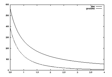
Consider round wafers, 20 cm in diameter, each costing $3500 to make. The total area of the wafer is about 315 square cm. If we choose to divide the wafer into roughly square dies of area a, we can fit about
315/a - 20pi/sqrt(2a)dies on it. The extra subtracted term accounts for the wasted area around the circumference of the circular wafer.
Die yield is the probability that an individual die is usable. Hennessy and Patterson approximate a typical yield by
(1+0.27*a)^(-3)The power of 3 comes from the three layers of silicon, polysilicon, and metal, in each of which there is some chance of failure. Hennessy and Patterson don't explain the probabilistic reasons for this formula. It is probably only valid for areas fairly near to 1 square centimeter. For very large areas, the probability of usability should be exponential, based on nearly independent chances for failure at each point on the wafer. We'll just trust the formula for now.
We could fit one large square die of 200 square centimeters on our 20-centimeter wafer. Why don't we? According to the formula, the yield would be about 6x10^(-6), so only one in 160,000 wafer-sized dies would be free of error. Each good die would cost over $500 million. The yield formula may not be precise for such a large die area, but it is probably an overestimate. In any case, it's clear that we can't make our dies that big.
On the other hand, we can fit 269 1 square centimeter dies, with a yield of 49%, so 132 of them are good, and they cost $27 each. Or, we can fit 107 2.25 square centimeter dies, with a yield of 24%, so 25 of them are good, and they cost $140 each. We can only justify 2.25 square centimeter dies if they are at least 5 times as valuable as 1 square centimeter dies. We can put all the circuitry of one 2.25 square centimeter die on three dies of 1 square centimeter each, with plenty of room for external connectors around the edge. So, the 5-times advantage of a larger die must come from the greater speed of communication on one chip vs. between chips.
Here is a plot of the number of dies, and the number of good dies,
per wafer as die area goes from 0.5 to 4 square centimeters.
To pick a die size, we need the value of different sizes, so we can compute the profit in making chips. There is usually no way to determine this value precisely, but we can make some estimates. It will typically go up in steps, as we reach sizes that allow particular desirable designs to fit on the chip. For the sake of example, suppose that in the range from 1/2 to 4 square centimeters, the value of a die is roughly
(a-0.4)60That is, we need 0.4 square centimeters to do anything useful at all, and then we can increase the value of our design by $60 for each additional square centimeter. Here is a graph of the cost per die and the value per die:
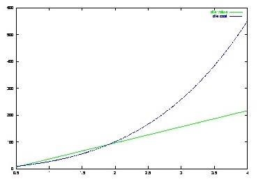
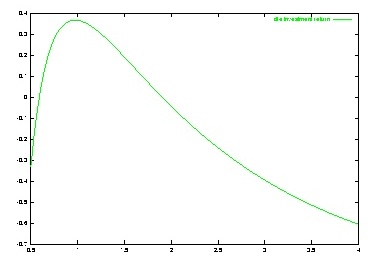
Chip designers probably don't draw these curves explicitly. More likely, they estimate the area required to implement some new feature, and then ask whether that feature is worth the cost increment.
Most books and articles present circuit design problems in the form, ``What is the best (fastest, smallest) circuit to accomplish the function f?'' Solutions to such problems, particularly for widely useful functions, such as memory and ALU, are very useful. But, a hardware designer is often faced with what I call a ``backwards'' problem: ``What is the most valuable circuitry that I can fit on a single die?'' Similar backwards problems arise at other levels of packaging, such as a single board, a single desktop pedestal, and in dimensions other than space, such as, ``What is the most valuable computation that I can accomplish on my disk controller during one rotation of the disk?'' A theoretical study of backward design would be very interesting, and worthy of several Ph.D. degrees. For example, find a sensible definition of the power of a finite-state machine, and solve the problem: ``Given i, o, and s, what is the most powerful finite-state machine with i input symbols, o output symbols, and s states?''
Computer design is full of little optimization problems, like the one above to choose the best die size. Textbook presentation of such problems can make each one look fairly easy. The hard part is the way they interact. I can't present the actual complexity of the interaction of different considerations in computer design, but I'll try to give a qualitative sense of the nature of the complexity.
Lots of industrial problems are expressed in terms of linear programming. The word ``linear'' suggests something easy, but linear programming is very hard, because it's not really linear but only piecewise linear. The word ``programming'' is also misleading: this is a type of mathematical problem, not a form of programming in the sense that you are familiar with in C, Pascal, Scheme, etc.
For example, here is a tiny fictional linear programming problem, having to do with the arithmetic and memory speed in a computer. Since I made it up, the specific numbers may not be realistic.
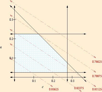
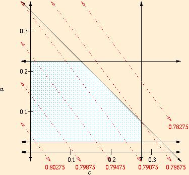
In linear programming, and in other even more complicated
optimization problems, the solution always occurs at an extreme corner
point. Small changes to the constraints and/or objective function may
send the solution to a distant corner. For example, if we find a new
cache design taking half the space of our old design, the objective
function might change to 0.8 - 0.03a - 0.04c, as shown
below. A similar change to the objective function could result from
optimizing a program with more memory accesses and fewer arithmetic
operations.
Real problems in computer architecture may easily have dozens of variables, and the dimension of the picture is the number of variables. The shapes of regions defined by linear constraints are called ``simplexes.'' Linear programming appears to be computationally difficult because the number of corners on a simplex grows exponentially with the number of variables.
The most unrealistic part of the example above is that the objective function for instruction time as a function of ALU area and cache area is surely not linear. But, nonlinear constraints and objective functions just make things even more complicated. The sort of jumping from one corner to another in the example above is very realistic.
Simple optimization problems, such as the optimization of die size in the previous section, correspond roughly to optimization near one corner of a simplex. The pattern of constraints and parameters around the solution to an optimization problem are called the ``limiting factors.'' Life is complicated, not just because constraints and objectives are sometimes complicated, but moreso because we focus attention on the current limiting factors, and small changes in the world shift them completely. In the linear programming example above, the limiting factor shifted suddenly from ALU size to cache size. Notice that engineering projects, including computer design, change the constraints and objective functions at the same time that they optimize parameters.
In any given computer architecture, with a particular programming load, there tends to be one element that limits the speed of the whole system. It could be network interface, disk, memory, the bus, part of the ALU, .... A good way to improve performance is to identify the bottleneck component, and speed it up. But, at some point this chosen component ceases to be the bottleneck, the whole structure of the system load changes, and a new bottleneck arises. At this point, further improvement in the original bottleneck component yields little or no benefit. Changes of performance bottleneck are particularly common examples of the sudden shifting of limiting factors in optimization problems.
Read 1.5 fairly carefully. The crucial point is that clear, accurate, and general performance comparisons are impossible, but we have to do them anyway.
Although computer performance is essentially a question of time, there are two components of time performance that usually need to be separated: throughput and latency. The distinction between throughput and latency performance arises whenever a computing system or component performs a sequence of similar tasks.
In the text, the phrases ``response time,'' ``wall-clock time,'' ``elapsed time,'' ``CPU time,'' all refer to latency. ``Bandwidth'' refers to throughput of a communication channel.
Another key concept in understanding performance is overhead. Overhead is work that is added to make a whole system work, even though it is not demanded by the required end result. For example, when we send a message on a network, we usually need to add some header describing the message and helping the network devices to route it, and we may need to padd the message to reach some standard size that the network devices work with. All bits added to the initial message are overhead. The distinction between overhead and required work depends on point of view, and the different views of overhead lead to different reports of throughput. For example, the throughput of an e-mail system should count the number of characters typed by the users that are transmitted per second, while the throughput of the underlying network mechanism should count all the bits in messages emitted by the e-mail system, many of which are overhead at the e-mail level. From the point of view of a numerical program, time used in executing the operating system is often considered overhead. In the 60s, computer centers often regarded everything other than floating point multiplications as CPU overhead. Because of overhead, throughput usually looks better at lower levels of abstraction in a system, although data compression occasionally reverses that effect.
In the text, ``user CPU time'' is nonoverhead, and other CPU time is overhead.
The quality of a measurement has two different components that are often confused: precision (also called resolution) and accuracy.
Although throughput of subsystems and components is a crucial issue in the performance of a system, the bottom line is usually latency for a whole task. All of the discussion in 1.5 is concerned with the problem of measuring latency, although the results are sometimes reported as speed, where speed = 1/latency. In spite of the fact that the performance of real work depends on a whole system, we have to choose components of our system, so we can't avoid some sort of comparative measure of computer performance when we decide which computer to buy. A measure of performance is very valuable as long as it leads to a sensible decision, even if it is neither precise nor accurate.
Computer performance is generally measured by timing computations on standard ``benchmark'' suites of programs. Taken with enough grains of salt, benchmark timings are very useful in evaluating the quality of computers. The grains of salt include:
With all their faults, benchmarks are what we've got to help us choose computers. Some vendors also report ``peak speeds.'' These are speeds that part of the computer can maintain assuming that it never waits for other components. Ignore ``peak speed'' reports, since they seldom have anything serious to do with useful performance.
Read 1.6 carefully.
Almost all clever ideas for improving computer performance follow from four (not completely independent) principles:
1 & 2 are also dangerous principles, since changes to one part of a system (particularly to software) can change the bottleneck and violate patterns of behavior thought to be common. Overdependence on these principles in one part of a system can inhibit flexibility in other parts. For example, most processors now use instruction pipelining, because execution of instructions in sequence is a common pattern of behavior. Typical pipelined architectures ruin the efficiency of a very clever idea that uses run-time modification of code to speed the evaluation of complex expressions.
Once it's stated in a simple form, Amdahl's law sounds trivial:
If task A takes time t, improvements to task A cannot save more than time t.But, remarkably smart people have wasted efforts due to overlooking implications of this rule. Read the statement in the text carefully. The law requires a sensible interpretation of ``task,'' such as the ``execution mode'' described in the text. The presentation of Amdahl's law in the text merely recasts the simple form above in terms of percentage speedups.
Amdahl's law is a sort of ``law of diminishing returns.'' As we speed up a task, the percentage improvement in terms of total latency diminishes. (On the other hand, the potential for large percentage improvement by speeding up other tasks increases.) The surprising quality of Amdahl's law, and the sense of diminishing returns, results entirely from the consideration of percentage improvement, instead of absolute time. Notice that the diminishing returns in bottleneck behavior is much more severe, and applies to absolute time.
The behavior described in Amdahl's law is most directly associated with latency measurements, since overall latency results is typically the sum of latency due to different steps. The more extreme sort of diminishing returns described in the notes on linear programming above, and associated with changing bottlenecks, is most directly associated with throughput measurements. But, throughput and latency measurements interact quite a bit. For example, the latency of a program that executes a lot of additions may depend on the throughput of the ALU. The throughput of a system typically depends on the latency of a bottleneck component.
We will look at memory hierarchy more carefully in Chapter 5. For now, read through 1.7 and identify the occurrence of concepts from 1.1-1.6 and from my notes above. Hennessy and Patterson are very explicit about the use of common patterns of behavior in the memory hierarchy, but in what way do cache and virtual memory exploit overlapping latency? In the conventional 5 (or is it 4?) components of a computer, one component is ``memory.'' Which levels of the memory hierarchy correspond to ``memory'' in the conventional view? Is there some room for variation in drawing the boundaries of conventional ``memory''? Suppose that registers and cache had exactly the same speed, but you were only allowed to choose one or the other, not both. What considerations would favor registers, what considerations would favor cache? Assume that you definitely have registers: how does the presence or absence of cache interact with the choice of register-register operations vs. memory-memory operations?
Read 1.8 carefully. Make sure that you understand precisely what is wrong with each fallacy and pitfall.
1.9 isn't crucial to us, but it's short and easy.
Read 1.10 for fun. Hennessy and Patterson omitted one of the most interesting historical facts about computing: the identity of the first company to sell a computer to another company. It was a British pastry company. If you can discover the name of the company, and/or any interesting details, please post.
Hennessy and Patterson point out very explicitly that, although we are studying hardware architecture in this class, the ``bottom line'' in performance is the behavior of the whole system of software application, compiler, operating system, architecture, and electronics. People recognized some time ago that particular computational problems can often be solved in more than one of these components, and deciding which is a tricky problem. Given unlimited design effort, there's a sense in which a hardware solution can always perform at least as well as a software solution to the same problem. Nonetheless, several attempts to solve problems efficiently in hardware have failed.
Computer scientists at Emory University noticed that special-purpose circuitry could speed up some of the mathematical operations required for factoring large integers very substantially, and could carry out portions of factoring algorithms in parallel. They designed and fabricated the Georgia Cracker machine containing their special VLSI circuits. But, an informal coalition of stock desktop workstations, communicating across the Internet, achieved better performance. What happened? During the time that the small project team at Emory was doing their work, a huge army of people at Intel, Motorola, etc. were improving the underlying electronic technology, and designing new processor and memory chips to exploit it. In addition to greater numbers, they had the advantage of making incremental changes to previous designs, instead of creating from scratch. By the time the Georgia Cracker was finished, it performed better than software on general-purpose machines from the time when the project started, but not as well as software on the networks of general-purpose machines that were available when they finished. In many ways, computer work is a race, and success depends not only on how well you do, but on how quickly you do it.
Another economic principle appears out of the Cracker case. Just as investment sharks use other people's money to get rich, computer engineers use other people's (hardware and software) work to solve their own problems. Computing is a thoroughly communal business. The main determinant of success is often not the quality of one's own work, in isolation, but rather the effectiveness with which it exploits the latest work by thousands of other people around the world.
Surely some day, the technological background for computing must stabilize. On that strange day, will we see a greater variety of special-purpose circuitry? My analysis above suggests that one of the pressures against special-purpose circuitry will diminish, but will others appear?
![[]](http://cs-www.uchicago.edu/images/misc/lightningbolt2.gif) odonnell@cs.uchicago.edu
odonnell@cs.uchicago.edu